Tag: machine learning

Splunk is a software platform designed to search, analyze and visualize machine-generated data, making sense of what, to most of us, looks like chaos.

Ordinarily, the machine data used by Splunk is gathered from websites, applications, servers, network equipment, sensors, IoT (internet-of-things) devices, etc, but there’s no limit to the complexity of data Splunk can consume.

Splunk specializes in Big Data, so why not use it to search the biggest data of all and find exoplanets?

What is an exoplanet?

An exoplanet is a planet in orbit around another star.

The first confirmed exoplanet was discovered in 1995 orbiting the star 51 Pegasi, which makes this an exciting new, emerging field of astronomy. Since then, Earth-based and space-based telescopes such as Kepler have been used to detect thousands of planets around other stars.

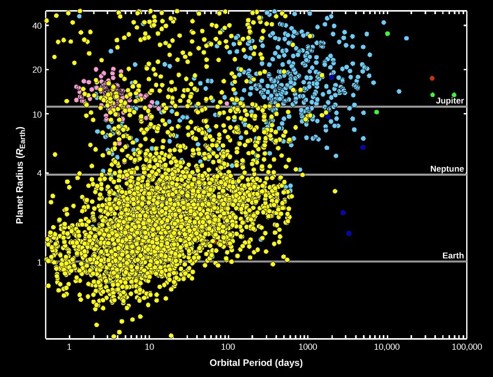
At first, the only planets we found were super-hot Jupiters, enormous gas giants orbiting close to their host stars. As techniques have been refined, thousands of exoplanets have been discovered at all sizes and out to distances comparable with planets in our own solar system. We have even discovered exomoons!

How do you find an exoplanet?

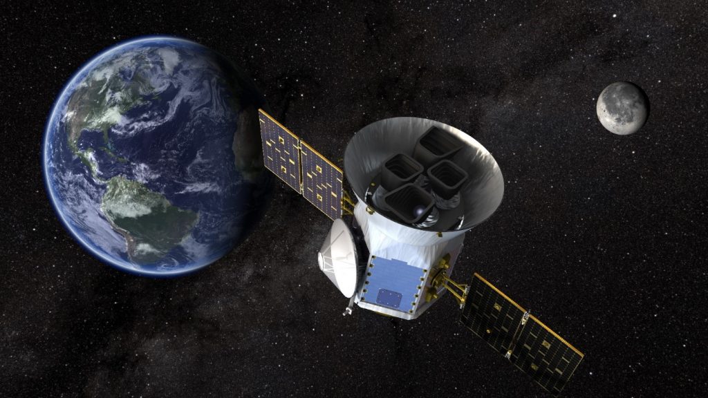
Imagine standing on stage at a rock concert, peering toward the back of the auditorium, staring straight at one of the spotlights. Now, try to figure out when a mosquito flies past that blinding light. In essence, that’s what telescopes like NASA’s TESS (Transiting Exoplanet Survey Satellite) are doing.

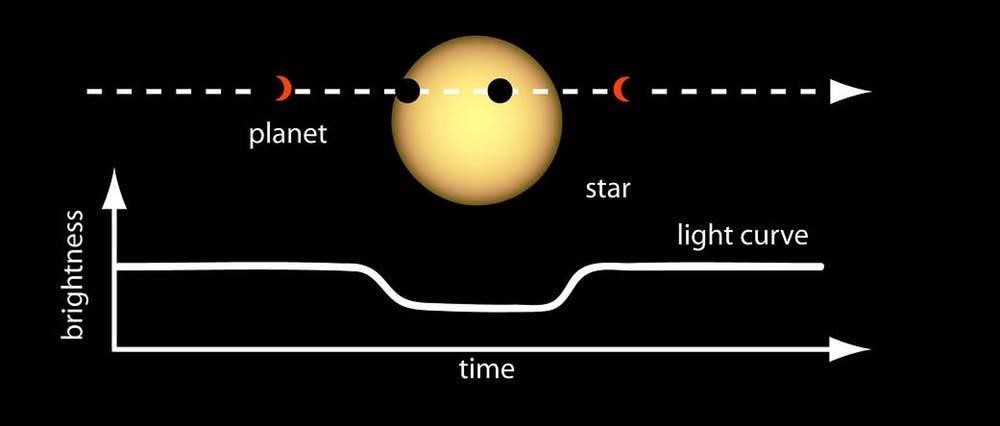
The dip in starlight intensity can be just a fraction of a percent, but it’s enough to signal that a planet is transiting the star.

Transits have been observed for hundreds of years in one form or another, but only recently has this idea been applied outside our solar system.

Australia has a long history of human exploration, starting some 60,000 years ago. In 1769 after (the then) Lieutenant James Cook sailed to Tahiti to observe the transit of Venus across the face of the our closest star, the Sun, he was ordered to begin a new search for the Great Southern Land which we know as Australia. Cook’s observation of the transit of Venus used largely the same technique as NASA’s Hubble, Kepler and TESS space telescopes but on a much simpler scale.

Our ability to monitor planetary transits has improved considerably since the 1700s.

NASA’s TESS orbiting telescope can cover an area 400 times as broad as NASA’s Kepler space telescope and is capable of monitoring a wider range of star types than Kepler, so we are on the verge of finding tens of thousands of exoplanets, some of which may contain life!

How can we use Splunk to find an exoplanet?

 Science thrives on open data.

All the raw information captured by both Earth-based and space-based telescopes like TESS are publicly available, but there’s a mountain of data to sift through and it’s difficult to spot needles in this celestial haystack, making this an ideal problem for Splunk to solve.

While playing with this over Christmas, I used the NASA Exoplanet Archive, and specifically the PhotoMetric data containing 642 light curves to look for exoplanets. I used wget in Linux to retrieve the raw data as text files, but it is possible to retrieve this data via web services.

MAST, the Mikulski Archive for Space Telescopes, has made available a web API that allows up to 500,000 records to be retrieved at a time using JSON format, making the data even more accessible to Splunk.

Some examples of API queries that can be run against the MAST are:

• List mission names
• Find the location of a star by name or ID
• Retrieve a list of all the stars in a search radius of just 0.2 degrees when looking at a certain celestial location

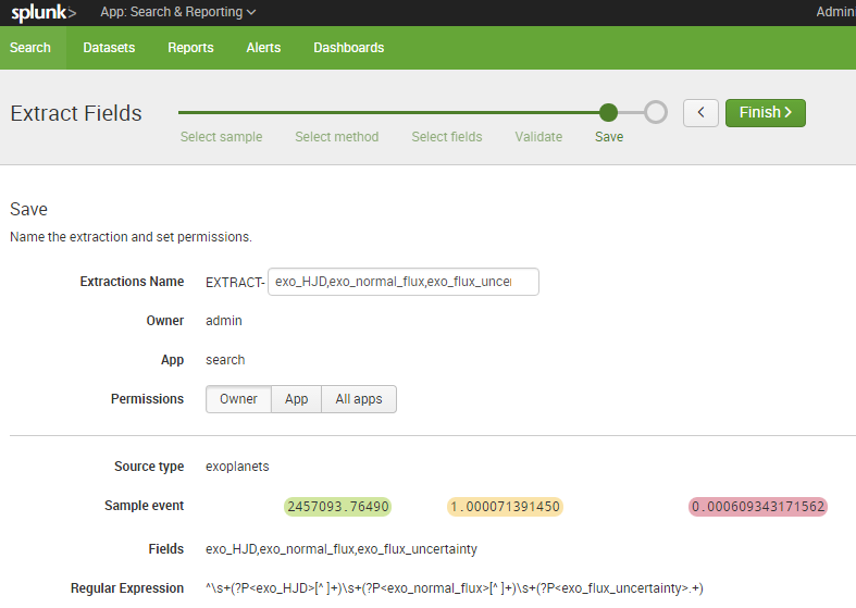
The raw data for a given observation appears as:

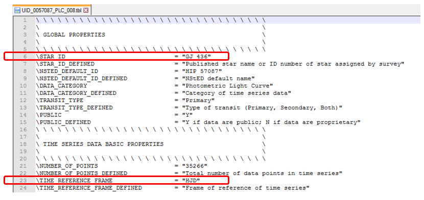
Information from the various telescopes does differ in format and structure, but it’s all stored in text files that can be interrogated by Splunk.

Values like the name of the star (in this case, Gliese 436) are identified in the header, while dates are stored either using HJD (Heliocentric Julian Dates) or BJD (Barycentric Julian Dates) centering on the Sun (with a difference of only 4 seconds between them).

Some observatories will use MJD which is the Modified Julian Date (being the Julian Date minus 2,400,000.5 which equates to November 17, 1858). Sounds complicated, but MJD is an attempt to simplify date calculations.

Think of HJD, BJD and MJD like UTC but for the entire solar system.

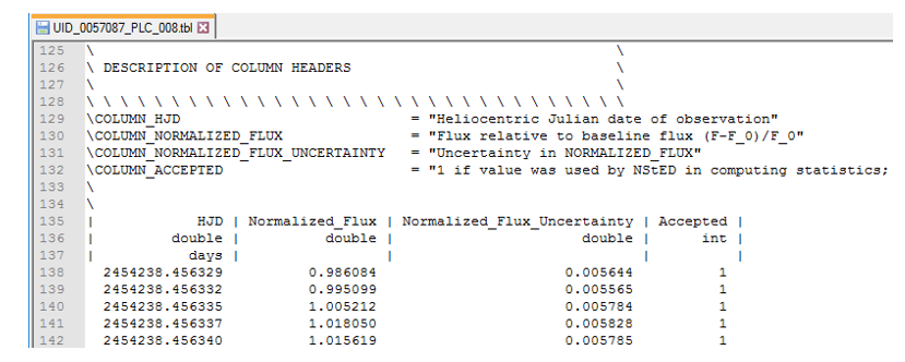
One of the challenges faced in gathering this data is that the column metadata is split over three lines, with the title, the data type and the measurement unit all appearing on separate lines.

The actual data captured by the telescope doesn’t start being displayed until line 138 (and this changes from file to file as various telescopes and observation sets have different amounts of associated metadata).

In this example, our columns are…

• HJD - which is expressed as days, with the values beyond the decimal point being the fraction of that day when the observation occurred
• Normalized Flux - which is the apparent brightness of the star
• Normalized Flux Uncertainty - capturing any potential anomalies detected during the collection process that might cast doubt on the result (so long as this is insignificant it can be ignored).

Heliocentric Julian Dates (HJD) are measured from noon (instead of midnight) on 1 January 4713 BC and are represented by numbers into the millions, like 2,455,059.6261813 where the integer is the days elapsed since then, while the decimal fraction is the portion of the day. With a ratio of 0.00001 to 0.864 seconds, multiplying the fraction by 86400 will give us the seconds elapsed since noon on any given Julian Day. Confused? Well, your computer won’t be as it loves working in decimals and fractions, so although this system may seem counterintuitive, it makes date calculations simple math.

We can reverse engineer Epoch dates and regular dates from HJD/BJD, giving Splunk something to work with other than obscure heliocentric dates.

• As Julian Dates start at noon rather than midnight, all our calculations are shifted by half a day to align with Epoch (Unix time)
• The Julian date for the start of Epoch on CE 1970 January 1st 00:00:00.0 UT is 2440587.500000
• Any-Julian-Date-minus-Epoch = 2455059.6261813 - 2440587.5 = 14472.12618
• Epoch-Day = floor(Any-Julian-Date-minus-Epoch) * milliseconds-in-a-day = 14472 * 86400000 = 1250380800000
• Epoch-Time = floor((Any-Julian-Date-minus-Epoch – floor(Any-Julian-Date-minus-Epoch)) * milliseconds-in-a-day = floor(0. 6261813 * 86400000) = 10902064
• Observation-Epoch-Day-Time = Epoch-Day + Epoch-Time = 1250380800000 + 10902064 = 1250391702064

That might seem a little convoluted, but we now have a way of translating astronomical date/times into something Splunk can understand.

I added a bunch of date calculations like this to my props.conf file so dates would appear more naturally within Splunk.

[exoplanets]

SHOULD_LINEMERGE = false

LINE_BREAKER = ([\r\n]+)

EVAL-exo_observation_epoch = ((FLOOR(exo_HJD - 2440587.5) * 86400000) + FLOOR(((exo_HJD - 2440587.5) - FLOOR(exo_HJD - 2440587.5))  *  86400000))

EVAL-exo_observation_date = (strftime(((FLOOR(exo_HJD - 2440587.5) * 86400000) + FLOOR(((exo_HJD - 2440587.5) - FLOOR(exo_HJD - 2440587.5))  *  86400000)) / 1000,"%d/%m/%Y %H:%M:%S.%3N"))

EVAL-_time = strptime((strftime(((FLOOR(exo_HJD - 2440587.5) * 86400000) + FLOOR(((exo_HJD - 2440587.5) - FLOOR(exo_HJD - 2440587.5))  *  86400000)) / 1000,"%d/%m/%Y %H:%M:%S.%3N")),"%d/%m/%Y %H:%M:%S.%3N")

Once date conversions are in place, we can start crafting queries that map the relative flux of a star and allow us to observe exoplanets in another solar system.

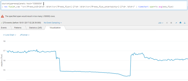
Let’s look at a star with the unassuming ID 0300059.

sourcetype=exoplanets host="0300059"

| rex field=_raw "\s+(?P<exo_HJD>24\d+.\d+)\s+(?P<exo_flux>[-]?\d+.\d+)\s+(?P<exo_flux_uncertainty>[-]?\d+.\d+)" | timechart span=1s avg(exo_flux)

And there it is… an exoplanet blotting out a small fraction of starlight as it passes between us and its host star!

What about us?

While curating the Twitter account @RealScientists, Dr. Jessie Christiansen made the point that we only see planets transit stars like this if they’re orbiting on the same plane we’re observing. She also pointed out that “if you were an alien civilization looking at our solar system, and you were lined up just right, every 365 days you would see a (very tiny! 0.01%!!) dip in the brightness that would last for 10 hours or so. That would be Earth!”

There have even been direct observations of planets in orbit around stars, looking down from above (or up from beneath depending on your vantage point). With the next generation of space telescopes, like the James Webb, we’ll be able to see these in greater detail.

Image credit: NASA exoplanet exploration

Next steps

From here, the sky’s the limit—quite literally.

Now we’ve brought data into Splunk we can begin to examine trends over time.

Astronomy is BIG DATA in all caps. The Square Kilometer Array (SKA), which comes on line in 2020, will create more data each day than is produced on the Internet in a year!

Astronomical data is the biggest of the Big Data sets and that poses a problem for scientists. There’s so much data it is impossible to mine it all thoroughly. This has led to the emergence of citizen science, where regular people can contribute to scientific discoveries using tools like Splunk.

Most stars have multiple planets, so some complex math is required to distinguish between them, looking at the frequency, magnitude and duration of their transits to identify them individually. Over the course of billions of years, the motion of planets around a star fall into a pattern known as orbital resonance, which is something that can be predicted and tested by Splunk to distinguish between planets and even be used to predict undetected planets!

Then there’s the tantalizing possibility of exomoons orbiting exoplanets. These moons would appear as a slight dip in the transit line (similar to what’s seen above at the end of the exoplanet’s transit). But confirming the existence of an exomoon relies on repeated observations, clearly distinguished from the motion of other planets around that star. Once isolated, the transit lines should show a dip in different locations for different transits (revealing how the exomoon is swinging out to the side of the planet and increasing the amount of light being blocked at that point).

Given its strength with modelling data, predictive analytics and machine learning, Splunk is an ideal platform to support the search for exoplanets.